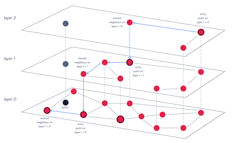
- What is High-Performance Vector Search & Graph-Based Retrieval Systems?
- Architectural Foundations of Active Nearest-Neighbor Learning
- Comparative Analysis: Active Metric Learning vs. Industry Alternatives
- Mathematical Intuition and Generalization Guarantees
- Deep Architectural Breakdown & Implementation Realities
- Critical Evaluation & Real-World Trade-Offs
- Adoption Guide: When to Adopt vs When to Pass
What is High-Performance Vector Search & Graph-Based Retrieval Systems?
High-Performance Vector Search & Graph-Based Retrieval Systems is a computational framework for indexing, querying, and classifying high-dimensional representations and metric spaces efficiently. It combines graph topologies, inverted indexes, and active learning algorithms to achieve sub-millisecond similarity search and accurate non-parametric classification across massive unstructured datasets.
To understand the necessity of advanced active learning architectures in metric spaces, we must first examine how vector retrieval and nearest-neighbor classification operate at scale. Traditional vector search frameworks rely on passive learning paradigms, where an algorithm ingests an exhaustively labeled training set to construct a static index or decision boundary. In high-dimensional spaces—such as those generated by transformer-based language models or deep convolutional neural networks—obtaining manual labels for millions of high-dimensional data points is prohibitively expensive and time-consuming.
Metric spaces generalize standard Euclidean spaces by defining a distance function that satisfies symmetry, identity of indiscernibles, and the triangle inequality. By shifting the operational paradigm from passive supervision to active metric learning, systems can selectively query only the most informative data points from a pool. This drastically cuts down annotation costs while maintaining tight theoretical bounds on generalization error.
Architectural Foundations of Active Nearest-Neighbor Learning
Active nearest-neighbor learning architectures minimize label complexity by intelligently selecting pool samples near classification boundaries, leveraging margin regularization to suppress noise in high-dimensional metric spaces. When building high-performance retrieval systems, engineering teams must balance computational query latency, index memory footprint, and labeling budgets.
The core philosophy of margin-regularized metric active learning (such as the MARMANN algorithm) centers on two primary components: a generalized sample compression scheme and an active model-selection mechanism. In a standard pool-based active learning setup, the learner has access to a large, unlabeled pool of metric-space instances. Rather than querying labels uniformly at random or processing every instance, the active learner evaluates the margin of uncertainty for candidate points.
Data points that lie deep within a homogeneous cluster provide negligible marginal utility because their nearest-neighbor classification is already overwhelmingly certain. Conversely, data points situated close to decision boundaries—where classes intersect or overlap—carry high epistemic uncertainty. By targeting these boundary regions, the active learner acquires labels only where they maximally constrain the resulting nearest-neighbor decision boundary.
From a systems engineering perspective, implementing this architecture requires a decoupled storage and compute topology. Unlabeled vector pools are indexed using approximate nearest neighbor (ANN) graph structures or metric trees to enable rapid spatial queries, while a lightweight active selection controller orchestrates label requests.
import numpy as np
from typing import Callable, List, Tuple

class MetricSpaceActiveLearner:
    def __init__(self, distance_metric: Callable[[np.ndarray, np.ndarray], float], margin_threshold: float):
        self.distance_metric = distance_metric
        self.margin_threshold = margin_threshold
        self.labeled_pool_x: List[np.ndarray] = []
        self.labeled_pool_y: List[int] = []

    def compute_metric_neighborhood(self, query_point: np.ndarray, candidate_pool: List[np.ndarray]) -> List[Tuple[float, int]]:
        distances = []
        for idx, candidate in enumerate(candidate_pool):
            dist = self.distance_metric(query_point, candidate)
            distances.append((dist, idx))
        distances.sort(key=lambda x: x[0])
        return distances

    def select_informative_samples(self, unlabelled_pool: List[np.ndarray], budget: int) -> List[int]:
        selected_indices = []
        for idx, point in enumerate(unlabelled_pool):
            if len(selected_indices) >= budget:
                break
            # Evaluate margin uncertainty heuristic
            if self.is_near_boundary(point):
                selected_indices.append(idx)
        return selected_indices

    def is_near_boundary(self, point: np.ndarray) -> bool:
        if not self.labeled_pool_x:
            return True
        neighbors = self.compute_metric_neighborhood(point, self.labeled_pool_x)
        if len(neighbors) < 2:
            return True
        nearest_dist, _ = neighbors[0]
        second_nearest_dist, _ = neighbors[1]
        margin = abs(nearest_dist - second_nearest_dist)
        return margin < self.margin_threshold
Comparative Analysis: Active Metric Learning vs. Industry Alternatives
Evaluating active metric learning against traditional vector search and passive classification paradigms highlights distinct trade-offs in labeling cost, compute complexity, and retrieval accuracy across distributed production environments.
| Approach / Design | Latency / Throughput | Computational & Resource Complexity | Maturity | Best For |
|---|---|---|---|---|
| Active Metric Learning (MARMANN) | Moderate query latency; highly optimized for low label complexity. | O(N log N) index construction; iterative distance evaluations during active pool sampling. | Academic / Advanced R&D | High labeling cost domains, custom metric spaces (strings, trees, graphs). |
| Passive Nearest Neighbor (Standard k-NN) | Sub-millisecond via HNSW or IVF indexes; high memory footprint. | O(N) search time without indexes; intensive memory requirements for raw vectors. | Industry Standard | Abundantly labeled datasets, standard Euclidean vector retrieval. |
| Deep Metric Learning (Contrastive / Triplet Nets) | Extremely fast inference using pre-trained dense embeddings. | High GPU training overhead; requires massive batch curation. | Production Mainstream | Semantic search, image retrieval, large-scale recommendation engines. |
Mathematical Intuition and Generalization Guarantees
Understanding the theoretical robustness of metric-space active learning requires analyzing sample compression bounds and noisy-margin properties without relying on rigid geometric assumptions.
In traditional machine learning, generalization error bounds are frequently derived for Euclidean spaces where linear boundaries or smooth manifolds are easy to construct. However, real-world data frequently resides in general metric spaces where the distance function satisfies only the metric axioms. The theoretical brilliance of margin-regularized active nearest-neighbor frameworks lies in their ability to yield prediction error guarantees that depend directly on the noisy-margin properties of the input sample.
Informally, the noisy-margin property measures the density of data points that reside close to the decision boundary relative to those that reside safely within their respective classes. When a dataset exhibits a favorable margin distribution—meaning very few points straddle the boundary—active learning algorithms can achieve exponential reductions in label complexity compared to passive learners.
The generalized sample compression scheme operates by demonstrating that any classifier output by the active learning algorithm can be reconstructed using a small subsample (the compression set) plus a small amount of auxiliary metadata. By binding the generalization error to the size of this compression set rather than the ambient dimension of the metric space, the theory bypasses the curse of dimensionality.
Deep Architectural Breakdown & Implementation Realities
Deploying metric-space active learning systems at production scale demands careful consideration of index synchronization, memory hierarchies, and concurrency control during active pool sampling iterations.
A production-grade vector search and active learning pipeline typically consists of three decoupled layers: 1. The Ingestion and Indexing Tier: Handles incoming high-dimensional vectors, maintaining approximate nearest-neighbor graphs (such as Hierarchical Navigable Small World graphs) or metric trees for fast distance calculations. 2. The Active Sampling Controller: Executes margin calculation heuristics against candidate pools, dispatching high-uncertainty items to human annotators or automated labeling oracles. 3. The Model Training & Evaluation Engine: Updates the compressed sample set and recalibrates distance metric weights as new labels stream into the system.
When implementing this pipeline, engineers frequently encounter performance bottlenecks related to distance metric evaluation. Computing pairwise distances across millions of pool items quickly saturates CPU memory bandwidth or GPU VRAM. To mitigate this, systems employ quantization techniques—such as Product Quantization (PQ) or Scalar Quantization (SQ)—to compress high-dimensional vectors into compact byte codes, enabling rapid approximate distance computations during the active selection phase.
class ProductionActiveRetrievalPipeline:
    def __init__(self, vector_dim: int, max_pool_size: int):
        self.vector_dim = vector_dim
        self.max_pool_size = max_pool_size
        self.unlabeled_pool = np.zeros((0, vector_dim), dtype=np.float32)
        self.labeled_pool = np.zeros((0, vector_dim), dtype=np.float32)
        self.labels = np.zeros((0,), dtype=np.int32)

    def ingest_batch(self, new_vectors: np.ndarray) -> None:
        if self.unlabeled_pool.shape[0] + new_vectors.shape[0] > self.max_pool_size:
            # Evict oldest unqueried vectors to maintain bounded memory
            overflow = (self.unlabeled_pool.shape[0] + new_vectors.shape[0]) - self.max_pool_size
            self.unlabeled_pool = self.unlabeled_pool[overflow:]
        self.unlabeled_pool = np.vstack([self.unlabeled_pool, new_vectors])

    def query_index_approximate(self, query: np.ndarray, k: int = 5) -> Tuple[np.ndarray, np.ndarray]:
        # Simulate approximate nearest neighbor search over labeled pool
        if self.labeled_pool.shape[0] == 0:
            raise ValueError("Labeled pool is empty. Initialize with active learning labels.")

        distances = np.linalg.norm(self.labeled_pool - query, axis=1)
        k = min(k, self.labeled_pool.shape[0])
        nearest_indices = np.argsort(distances)[:k]
        return distances[nearest_indices], self.labels[nearest_indices]
Critical Evaluation & Real-World Trade-Offs
While margin-regularized active nearest-neighbor algorithms provide strong theoretical guarantees and exceptional label efficiency, systems architects must weigh several practical limitations before adopting them in production.
First, the computational overhead of active pool sampling scales with the size of the unlabeled pool. Evaluating margin uncertainties across millions of high-dimensional points requires frequent nearest-neighbor searches, which can introduce latency spikes if executed synchronously on the primary serving thread. Consequently, active selection must run asynchronously as a background batch job.
Second, active learning algorithms are notoriously sensitive to label noise. Because active selection intentionally targets points near decision boundaries, an incorrect or noisy label assigned to a high-uncertainty boundary point can severely warp the local nearest-neighbor classifier. Production systems must incorporate robust validation filters and multi-annotator consensus mechanisms before accepting labels generated via active sampling.
Third, metric space generalization relies heavily on the quality of the underlying distance function. If the chosen metric fails to capture the true semantic similarity of the domain, even the most sophisticated active sampling strategy will produce suboptimal decision boundaries.
Adoption Guide: When to Adopt vs When to Pass
To determine whether to integrate active metric learning frameworks into your data architecture, evaluate your project against the following operational criteria:
- Adopt When: Label acquisition is extremely expensive, rare, or requires domain-expert human annotation (e.g., medical diagnostics, rare legal document classification, specialized fraud detection).
- Adopt When: Your data naturally resides in non-Euclidean metric spaces where standard parametric neural networks struggle, or where custom edit/kernel distances are required.
- Pass When: You have an abundance of cheap, pre-existing training labels and your primary bottleneck is raw query throughput rather than labeling budget.
- Pass When: Your system requires ultra-low-latency real-time online learning where model updates must occur within microseconds of a new interaction without background batch processing.
Frequently Asked Questions
What is the primary advantage of active nearest-neighbor learning over passive learning?
Active nearest-neighbor learning significantly reduces the number of training labels required to achieve a target prediction error by intelligently selecting and querying only the most informative data points near classification boundaries.
How does metric space independence benefit retrieval systems?
Metric space independence allows the underlying algorithm to operate over any valid distance function—including string edit distances, graph kernels, and non-Euclidean geometries—without being restricted to standard vector spaces.
What role does margin regularization play in classification performance?
Margin regularization ensures that decision boundaries maintain a robust separation from training instances, suppressing classification noise and improving generalization performance on unseen test data.
Why are generalized sample compression schemes important for theoretical guarantees?
Sample compression schemes prove that a classifier can be reconstructed from a small subset of the training data, allowing researchers to bound generalization error independently of the ambient dimensionality of the metric space.
How do approximate nearest neighbor (ANN) indexes integrate with active learning pools?
ANN indexes enable rapid spatial querying of unlabeled data pools, allowing the active learning controller to quickly locate boundary candidates and estimate local neighborhood margins without exhaustive pairwise scans.
What is the main operational challenge of pool-based active learning in production?
The primary challenge is managing the computational overhead of evaluating uncertainty metrics across massive unlabeled pools, which typically requires asynchronous background processing to avoid impacting query serving latency.
How does label noise impact active nearest-neighbor classifiers?
Because active learning specifically targets points near decision boundaries where classification is ambiguous, incorrect labels can disproportionately distort the local neighborhood structure and degrade overall accuracy.
When should an engineering team choose passive learning over active metric learning?
An engineering team should choose passive learning when high-quality training labels are already abundant and the primary system requirement is maximizing indexing and retrieval throughput with minimal algorithmic complexity.
How do vector quantization methods alleviate memory constraints during active pool sampling?
Quantization techniques compress high-dimensional vectors into compact byte codes, reducing memory bandwidth pressure and accelerating distance calculations during active selection phases.
What criteria should guide the selection of a distance metric in custom retrieval spaces?
Distance metrics should be chosen based on the underlying topology and domain semantics of the data, ensuring that metric axioms and semantic similarity measures are accurately preserved.