Direct Preference Optimization: Production Deep Dive

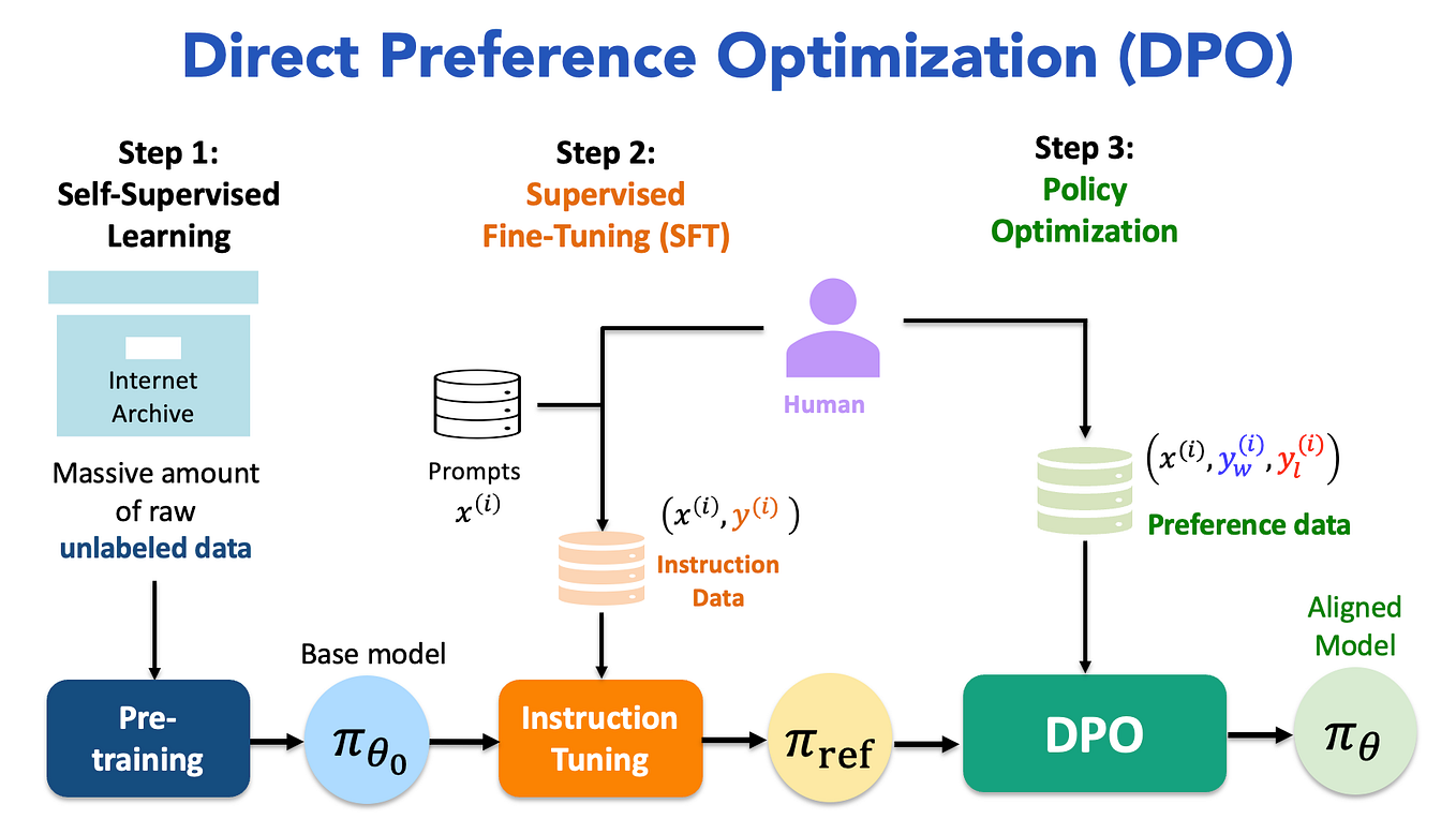
The quest to align large language models (LLMs) with human values, preferences, and safety constraints has historically relied on Reinforcement Learning from Human Feedback (RLHF). While highly effective, the traditional RLHF pipeline—exemplified by algorithms like Proximal Policy Optimization (PPO)—is notoriously complex, unstable, and resource-intensive, requiring the simultaneous coordination of up to four large models (actor, critic, reference, and reward models). In the landmark paper “Direct Preference Optimization: Your Language Model is Secretly a Reward Model,” Rafailov et al. introduce a radical mathematical reformulation that bypasses reward model training and reinforcement learning entirely. By proving that the optimal policy of a KL-constrained reinforcement learning objective can be derived in closed form, the authors demonstrate that LLMs can be aligned directly using a simple binary cross-entropy loss over preference pairs.

Key Technical & Architectural Takeaways

• Closed-Form Reward Elimination: DPO mathematically reformulates the RLHF objective to express the implicit reward function directly as a function of the language model’s policy and a frozen reference model, eliminating the need to train or infer a separate reward model.
• Elimination of the RL Loop: By transforming RL optimization into a supervised pairwise classification loss (binary cross-entropy), DPO eradicates the instability, extreme hyperparameter sensitivity, and high memory footprints associated with PPO’s actor-critic loops.
• Computational Efficiency: DPO cuts active memory overhead and training complexity significantly by reducing the active runtime model count from four (actor, critic, reference, reward) down to just two (policy and reference), while eliminating active online token generation during training.
• Mathematical Equivalence: DPO optimizes the exact same KL-constrained preference objective as traditional RLHF, but does so with a stable, deterministic gradient descent step that scales cleanly to frontier model regimes.

The Paradigm Shift: From PPO-RLHF to Direct Preference Optimization

Direct Preference Optimization (DPO) shifts the LLM alignment paradigm by replacing complex reinforcement learning loops with a simple, closed-form supervised classification loss. By mathematically equating the language model to its own implicit reward model, DPO bypasses reward model training, action-space sampling, and unstable actor-critic policy optimization.

To fully appreciate this breakthrough, we must first dissect the traditional RLHF pipeline, which operates in three distinct, sequential phases:

1. Supervised Fine-Tuning (SFT): Training a base model on high-quality, task-specific demonstrations to establish a base policy π^SFT. This phase is critical as it establishes the model’s command of language, syntax, and instruction-following formats. However, SFT alone is limited because it treats all tokens in the demonstration dataset with equal weight and does not capture human stylistic nuances or complex, multi-variable safety boundaries.
2. Reward Model Training: Collecting human preference datasets of the form D = (x, y_w, y_l), where x is a prompt, y_w is the preferred (winning) response, and y_l is the dispreferred (losing) response. A reward model r_ϕ(x, y) is trained to maximize the likelihood of the preferred responses under a choice model, typically the Bradley-Terry (BT) model:

   P(y_w succ y_l | x) = σ(r_ϕ(x, y_w) - r_ϕ(x, y_l))

   where σ(z) = 1 / (1 + e^-z) is the sigmoid function. This framework maps arbitrary human evaluations into a scalar utility space, ordering generations based on relative human preference.
3. Reinforcement Learning Optimization: Fine-tuning the SFT policy π_θ using a reinforcement learning algorithm (typically PPO) to maximize the reward r_ϕ(x, y) while penalizing divergence from the baseline SFT model via a Kullback-Leibler (KL) divergence term to prevent model collapse or reward hacking:

   Unlike classical PPO which requires optimizing a non-differentiable reinforcement learning reward via policy rollouts, Direct Preference Optimization (DPO) derives a closed-form solution for the optimal policy under the KL-constrained reward objective. By expressing the ground-truth reward implicitly through the ratio of the active policy to a reference policy, DPO cancels out the intractable partition function Z(x) entirely.

   The resulting DPO objective simplifies reinforcement learning into a stable, supervised binary cross-entropy loss over preference pairs (x, y_w, y_l):

   import torch
   import torch.nn.functional as F
   
   def compute_dpo_loss(
       policy_chosen_logps: torch.Tensor,
       policy_rejected_logps: torch.Tensor,
       reference_chosen_logps: torch.Tensor,
       reference_rejected_logps: torch.Tensor,
       beta: float = 0.1,
   ) -> torch.Tensor:
       """
       Direct Preference Optimization (DPO) Loss Function.
       Eliminates the separate reward model and actor-critic loops.
       """
       # Calculate log likelihood ratios between policy and frozen reference model
       pi_logratios = policy_chosen_logps - policy_rejected_logps
       ref_logratios = reference_chosen_logps - reference_rejected_logps
       
       # Scale difference by temperature parameter beta
       logits = beta * (pi_logratios - ref_logratios)
       
       # Binary cross-entropy loss over preference pairs
       losses = -F.logsigmoid(logits)
       return losses.mean()

   This direct formulation maps preference probabilities straight to policy updates. When the model assigns higher probability to preferred completions, the loss decreases smoothly without needing an actor-critic loop or reinforcement learning environment.

   L_DPO(π_θ; π_ref) = -E [ log σ ( β log fracπ_θ(y_w | x)π_ref(y_w | x) - β log fracπ_θ(y_l | x)π_ref(y_l | x) ) ]

   This formulation eliminates the need to train or evaluate a separate reward model. The language model π_θ acts as its own reward model during optimization. By optimizing this loss, the language model increases the relative likelihood of the preferred response y_w over the dispreferred response y_l, scaled by their respective ratios under the reference model π_ref.

   DPO Gradient Analysis and Optimization Dynamics

   DPO optimizes policy weights through gradient dynamics that mimic a self-regulating contrastive learning framework. By scaling the gradient updates with a dynamic sigmoid weighting factor, the model scales back gradient magnitude for already-aligned pairs while aggressively updating weights for incorrectly classified human preference samples, preventing gradient explosion.

   To understand why DPO is mathematically stable and self-regulating, we can analyze the gradient of the loss function mathcalL_DPO with respect to the policy parameters θ. Let us define the implicit reward estimate as:

   hatr_θ(x, y) = β log fracπ_θ(y | x)π_ref(y | x)

   Using this definition, the DPO loss can be written in a compact form:

   L_DPO(π_θ; π_ref) = -E [ log σ ( hatr_θ(x, y_w) - hatr_θ(x, y_l) ) ]

   Applying the chain rule to take the gradient with respect to the model parameters θ, we compute:

   ∇_θ L_DPO(π_θ; π_ref) = -β E [ σ(hatr_θ(x, y_l) - hatr_θ(x, y_w)) ( ∇_θ log π_θ(y_w | x) - ∇_θ log π_θ(y_l | x) ) ]

   This gradient formulation highlights two critical, self-regulating components that drive DPO’s stability and optimization dynamics:

   • The Likelihood Gradient Difference (∇_θ log π_θ(y_w | x) - ∇_θ log π_θ(y_l | x)): This component acts as a directional force. It pushes the model parameters to increase the log likelihood of the winning response y_w while simultaneously decreasing the log likelihood of the losing response y_l. It acts as a contrastive operator, forcing the model’s sequence space to draw clear boundaries around preferred behaviors.
   • The Dynamic Weighting Factor (σ(hatr_θ(x, y_l) - hatr_θ(x, y_w))): This term acts as an adaptive learning rate scaler. It measures how strongly the current model misclassifies the preference. If the model already assigns a much higher implicit reward to the winning response (hatr_θ(x, y_w) gg hatr_θ(x, y_l)), the term σ(hatr_θ(x, y_l) - hatr_θ(x, y_w)) approaches zero, and the gradient update becomes very small. Conversely, if the model currently misclassifies the preference (hatr_θ(x, y_l) > hatr_θ(x, y_w)), the weight approaches 1, applying a strong, corrective gradient update.

   This gradient-level analysis shows that DPO avoids the classic failure modes of unsupervised training and unconstrained optimization. By scaling the updates based on the current model’s alignment progress, it naturally mitigates gradient explosion and prevents over-correcting samples that have already been mastered. It acts as an implicit curriculum learning mechanism, naturally shifting optimization focus toward hard preference boundaries.

   Comparative Architecture: DPO vs. PPO vs. Industry Alternatives

   Direct Preference Optimization fundamentally differs from alternative alignment methods like PPO, KTO, and Rejection Sampling by directly optimizing preference likelihoods. It eliminates the multi-model complexity of PPO, avoids the massive inference sampling costs of Rejection Sampling, and implements a mathematically rigorous pairwise constraint that KTO simplifies into single-sample metrics.

   Choosing an alignment framework requires balancing training stability, memory overhead, and conversational performance. Two modern alternatives to consider are Kahneman-Tversky Optimization (KTO) and offline Rejection Sampling (often termed Best-of-N):

   • Kahneman-Tversky Optimization (KTO): Grounded in behavioral economics and prospect theory, KTO bypasses pairwise data requirements. Instead of comparing a preferred response directly to a dispreferred one, it evaluates isolated responses as either “good” or “bad” against a dynamic reference utility threshold. This makes data collection significantly cheaper, though it loses the sharp relative gradient signal that pairwise comparisons provide.
   • Rejection Sampling (Best-of-N): This brute-force alternative uses a frozen generator to sample N candidate responses for a given prompt, scores them all using a separate reward model, and selects the highest-scoring candidate. The generator is then fine-tuned on these chosen responses via standard Supervised Fine-Tuning (SFT). While simple, it does not allow the model to learn dynamically from its own structural mistakes during gradient updates, and has high runtime sampling costs.

   The following table provides a comprehensive technical comparison of these distinct paradigms:

   Dimension	DPO (Direct Preference Optimization)	PPO-RLHF (Proximal Policy Optimization)	KTO (Kahneman-Tversky Optimization)	Rejection Sampling (Best-of-N)
   Core Paradigm	Supervised closed-form binary classification over preference pairs.	Online Actor-Critic reinforcement learning with explicit reward.	Binary classification of single responses based on utility theory.	Offline sampling filtered by an external reward model.
   Data Requirements	Pairwise preferences: (x, y_w, y_l) pairs.	Pairwise preferences for Reward Model; prompts for RL.	Unpaired binary labels: (x, y, textgood/bad).	SFT data plus a separately trained reward model.
   Active Models in VRAM	2: Policy model (π_θ) & frozen Reference model (π_ref).	4: Policy, Reference, Reward (r_ϕ), and Critic (V_ψ).	2: Policy model (π_θ) & frozen Reference model (π_ref).	1 to 2: Generator model & Reward model (for offline filtering).
   Training Stability	High: Deterministic gradient descent, non-chaotic dynamics.	Low: Highly sensitive to learning rates, clipping, and init.	High: Extremely stable, behaves like binary classification.	High: Simple standard supervised fine-tuning (SFT) loop.
   Computational Complexity	Low: No online token generation; simple forward/backward passes.	Extremely High: Expensive active generation rollouts.	Low: No pairwise alignment; processes samples independently.	Medium-High: High inference cost to sample N candidates.
   Vulnerability to Reward Hacking	Low: Explicitly constrained by the β-KL margin backstop.	High: Policy easily exploits vulnerabilities in r_ϕ.	Low: Regulated via reference policy anchors.	Minimal: Limited strictly to the generated search space.
   Mathematical Foundation	Closed-form exact equivalence to KL-constrained RL.	Stochastic Policy Gradient approximation (PPO clipping).	Prospect Theory value functions with empirical thresholds.	Monte Carlo sampling combined with supervised behavior cloning.

   Deep Architectural Breakdown & Implementation Realities

   Implementing DPO in production requires managing critical memory and token-alignment challenges, specifically the simultaneous loading of active and reference policies. Engineers mitigate these hardware constraints using Low-Rank Adaptation (LoRA), reference log-probability caching for offline datasets, and custom sequence-packing mechanisms to handle pad-token masking and long contexts.

   To overcome this memory overhead in resource-constrained environments, engineers often combine DPO with parameter-efficient techniques like Low-Rank Adaptation (LoRA). By applying LoRA to the active policy, only the base model is loaded into VRAM alongside the active adapters. During the forward pass, the base model can be shared, or the reference log-probabilities can be pre-computed and cached if the dataset is entirely static. However, when using dynamic generation or on-the-fly training, keeping both models accessible remains the standard practice.

   Another major implementation hurdle is the computational processing of padded sequences. In standard autoregressive training, pad tokens are ignored in loss calculations. However, in DPO, a failure to correctly mask out pad tokens or prompt tokens when calculating sequence-level log probabilities will result in corrupt gradients, as the model attempts to optimize padding tokens. We must carefully compute the log probabilities only on the target response tokens, masking out both the prompt tokens and any sequence padding.

   The following list outlines the data flow during a single DPO optimization step:

   1. Batching Preference Pairs: The system feeds a prompt x along with both the winning response y_w and losing response y_l into the active policy π_θ and the frozen reference policy π_ref.
   2. Token Log-Probability Computation: The models perform forward passes to calculate the log probabilities of the target tokens for both generations under both policies. This yields four values: π_θ(y_w | x), π_θ(y_l | x), π_ref(y_w | x), and π_ref(y_l | x).
   3. Log-Ratio Comparison: The system computes the log-ratio of the active policy to the reference policy for both the winning and losing sequences. These ratios represent the implicit rewards.
   4. Loss Calculation & Backpropagation: The difference between these implicit rewards is scaled by the hyperparameter β, passed through a sigmoid function, and used to calculate the binary cross-entropy loss. Gradients are then backpropagated to update the active policy π_θ.

   The following production-grade PyTorch implementation demonstrates how to calculate the DPO loss, handle sequence padding, compute sequence-level log probabilities, and optimize the model parameters.

   import torch
   import torch.nn as nn
   import torch.nn.functional as F
   
   class DirectPreferenceLoss(nn.Module):
       """
       Direct Preference Optimization (DPO) Loss Module.
       Computes the binary cross-entropy loss over policy and reference log-ratios.
       """
       def __init__(self, beta: float = 0.1, label_smoothing: float = 0.0):
           super().__init__()
           self.beta = beta
           self.label_smoothing = label_smoothing
   
       def _get_batch_logps(
           self, 
           logits: torch.FloatTensor, 
           labels: torch.LongTensor, 
           attention_mask: torch.BoolTensor
       ) -> torch.FloatTensor:
           """
           Extracts token-level log-probabilities and sums them over the sequence.
           
           Args:
               logits: Tensor of shape (batch_size, sequence_length, vocabulary_size)
               labels: Tensor of shape (batch_size, sequence_length) with target tokens,
                       where non-target tokens (e.g., prompt tokens) are masked with -100.
               attention_mask: Tensor of shape (batch_size, sequence_length)
               
           Returns:
               log_probs: Tensor of shape (batch_size,) containing sequence-level log probabilities.
           """
           # Ensure logits and labels shapes align correctly
           assert logits.shape[0] == labels.shape[0], "Batch size mismatch between logits and labels."
           assert logits.shape[1] == labels.shape[1], "Sequence length mismatch between logits and labels."
   
           # Shift logits and labels by 1 step to match autoregressive generation targets
           shift_logits = logits[..., :-1, :].contiguous()
           shift_labels = labels[..., 1:].contiguous()
           shift_mask = attention_mask[..., 1:].contiguous()
   
           # Mask pad tokens and prompt tokens (conventionally marked with -100)
           loss_mask = shift_mask & (shift_labels != -100)
   
           # Replace masked labels with 0 to prevent index errors in gather operations
           dummy_labels = shift_labels.clone()
           dummy_labels[~loss_mask] = 0
   
           # Calculate log-softmax over vocabulary dimension
           log_probs = F.log_softmax(shift_logits, dim=-1)
           
           # Gather the log-probabilities of the actual target tokens
           per_token_logps = torch.gather(log_probs, dim=-1, index=dummy_labels.unsqueeze(-1)).squeeze(-1)
           
           # Sum the log-probabilities over the sequence dimension, applying the mask
           return (per_token_logps * loss_mask).sum(dim=-1)
   
       def forward(
           self,
           policy_chosen_logits: torch.FloatTensor,
           policy_rejected_logits: torch.FloatTensor,
           reference_chosen_logits: torch.FloatTensor,
           reference_rejected_logits: torch.FloatTensor,
           chosen_labels: torch.LongTensor,
           rejected_labels: torch.LongTensor,
           chosen_attention_mask: torch.BoolTensor,
           rejected_attention_mask: torch.BoolTensor
       ) -> tuple[torch.FloatTensor, torch.FloatTensor, torch.FloatTensor]:
           """
           Executes the DPO forward pass and calculates the preference loss.
           
           Args:
               policy_chosen_logits: Logits from active policy on chosen completions.
               policy_rejected_logits: Logits from active policy on rejected completions.
               reference_chosen_logits: Logits from reference policy on chosen completions.
               reference_rejected_logits: Logits from reference policy on rejected completions.
               chosen_labels: Target token IDs for chosen completions (prompt masked with -100).
               rejected_labels: Target token IDs for rejected completions (prompt masked with -100).
               chosen_attention_mask: Attention mask for chosen sequences.
               rejected_attention_mask: Attention mask for rejected sequences.
               
           Returns:
               losses: Scalar tensor representing the mean DPO loss across the batch.
               chosen_rewards: Detached tensor of implicit rewards for chosen sequences.
               rejected_rewards: Detached tensor of implicit rewards for rejected sequences.
           """
           # Compute log-probabilities for the policy model
           policy_chosen_logps = self._get_batch_logps(
               policy_chosen_logits, chosen_labels, chosen_attention_mask
           )
           policy_rejected_logps = self._get_batch_logps(
               policy_rejected_logits, rejected_labels, rejected_attention_mask
           )
   
           # Compute log-probabilities for the reference model
           with torch.no_grad():
               reference_chosen_logps = self._get_batch_logps(
                   reference_chosen_logits, chosen_labels, chosen_attention_mask
               )
               reference_rejected_logps = self._get_batch_logps(
                   reference_rejected_logits, rejected_labels, rejected_attention_mask
               )
   
           # Compute implicit rewards (log-ratios scaled by beta)
           chosen_log_ratios = policy_chosen_logps - reference_chosen_logps
           rejected_log_ratios = policy_rejected_logps - reference_rejected_logps
           logits = self.beta * (chosen_log_ratios - rejected_log_ratios)
   
           # Compute binary cross-entropy loss with optional label smoothing
           losses = (
               -F.logsigmoid(logits) * (1.0 - self.label_smoothing)
               - F.logsigmoid(-logits) * self.label_smoothing
           )
   
           # Track tracking metrics (implicit rewards for diagnostic logging)
           chosen_rewards = self.beta * chosen_log_ratios.detach()
           rejected_rewards = self.beta * rejected_log_ratios.detach()
   
           return losses.mean(), chosen_rewards, rejected_rewards

   Critical Evaluation & Real-World Trade-Offs

   Despite its stability and efficiency, DPO suffers from critical limitations including offline generalization bottlenecks, absolute likelihood decay, and sensitivity to noisy preference data. Because standard DPO lacks online exploration, policies easily overfit to training distributions, degrade in conversational capability, and collapse when trained on conflicting human labels.

   Three primary limitations impact the use of DPO in production:

   1. Overfitting to Offline Data & Loss of Distributional Control

   Unlike PPO, which continually samples fresh tokens (y sim π_θ) from the active policy during training to explore the response space, standard DPO is an offline algorithm. It evaluates log-likelihoods only on static sequences in the pre-collected dataset D. This lack of online exploration can lead to model degradation when there is a mismatch between the training data and real-world prompts.

   If the active policy’s generation distribution drifts too far from the reference policy π_ref, the model may struggle with out-of-distribution prompts, leading to repetitive generations or sudden drops in output quality. This behavior is often called “distributional drift” and is typically addressed in advanced pipelines by employing dynamic or iterative online generation variants (such as Iterative DPO or Online DPO), where fresh preferences are sampled and evaluated periodically during training.

   2. The “Likelihood Decay” Phenomenon

   Empirical research has shown that DPO can cause a phenomenon known as “likelihood decay” under high optimization epochs or poorly tuned β values. Although the relative log-ratio difference (r(x, y_w) - r(x, y_l)) increases as intended, the absolute log-probabilities of both responses can simultaneously decrease:

   log π_θ(y_w | x) → - ∈ fty quad and quad log π_θ(y_l | x) → - ∈ fty

   When this happens, the model shifts probability mass away from these target responses toward unaligned, out-of-distribution sequences. This degradation often manifests as gibberish outputs, repetitive punctuation, or severe model collapse, requiring strict early-stopping policies and careful tuning of the β regularizer.

   To combat this, engineers frequently add an auxiliary Supervised Fine-Tuning loss term back into the DPO objective. This joint optimization forces the model to maintain high absolute likelihood on the preferred responses, anchoring its underlying linguistic capabilities while it learns preference boundaries:

   L_Joint = L_DPO + α L_SFT

   3. Vulnerability to Noisy and Conflicting Preferences

   DPO relies on the assumption that human preferences align with the Bradley-Terry model. However, real-world preference data is often highly noisy, subjective, and self-contradicting. When faced with conflicting labels—such as when annotators disagree on subjective prompts—DPO’s gradient forces the model to balance conflicting log-probability updates.

   Unlike PPO, which benefits from the averaging effect of an explicit reward model that acts as an optimization buffer, DPO applies these noisy gradients directly to the policy. This direct update path makes DPO highly sensitive to mislabeled data, requiring rigorous data sanitization and label-filtering pipelines before training. When intransitive loops (e.g., response A is preferred to B, B is preferred to C, but C is preferred to A) exist in the data, DPO can enter local minima that degrade overall capabilities.

   Adoption Guide: When to Adopt vs. When to Pass

   Enterprise organizations should adopt DPO when prioritizing high training throughput, minimal GPU resource overhead, and leveraging curated, high-quality preference datasets. Conversely, teams should pass on DPO in favor of online reinforcement learning or rejection sampling when aligning complex, multi-step reasoning models that require active exploration.

   To assist engineering teams in making an architectural decision, the following guidelines direct the selection process based on specific computational, data, and hardware constraints.

   When to Adopt DPO

   • Accelerated Time-to-Market: You need to align models quickly without the long development and hyperparameter tuning cycles associated with PPO-RLHF.
   • Constrained Computational Budgets: You lack the GPU resources to run a four-model PPO stack (actor, critic, reference, reward) in parallel and want to avoid the high cost of generating active rollouts.
   • Static, Curated Preference Datasets: You have a clean, high-quality offline preference dataset that covers your production use cases well, minimizing the need for active exploration.
   • LoRA-Based Training Pipelines: Your infrastructure is optimized for Parameter-Efficient Fine-Tuning (PEFT), where a single base model can be shared between the active policy and the reference model.
   • Direct Style Alignment: Your primary goal is stylistic alignment, such as altering the tone, verbosity, formatting, or politeness of the generated responses.

   When to Pass (and Consider PPO or Rejection Sampling)

   • Open-Ended and Highly Complex Tasks: For tasks like multi-step mathematical reasoning, code execution, or interactive agent loops, online exploration is essential to discover optimal pathways.
   • Noisy or Automated Preference Signals: If your preference data is generated by weaker LLMs or crowdsourced with high error rates, training a separate reward model to act as a noise-filtering buffer is often more stable.
   • Strict Latency and Memory Constraints: If your training hardware cannot support loading both the active policy and the reference model simultaneously, and you cannot use pre-computed log probability caching.
   • Mathematical and Logical Rigor Constraints: When aligning models for factual correctness where the exact reward landscape is highly non-linear and sharp, which offline static datasets fail to map adequately.

   Strategic Architecture Conclusion & Production Roadmap

   Direct Preference Optimization (DPO) fundamentally redefines alignment architecture by collapsing the unstable, resource-intensive RLHF pipeline into a

   Frequently Asked Questions

   Is DPO mathematically identical to PPO?

   DPO is mathematically equivalent to the global optimal solution of the KL-constrained reinforcement learning objective optimized by PPO. However, their optimization paths differ in practice. PPO approaches this optimum using step-by-step policy gradient updates based on a dynamically changing policy, whereas DPO targets this optimum directly via a closed-form classification loss on static data.

   Why is the reference model necessary during DPO training?

   The reference model (π_ref) acts as a mathematical anchor to prevent the active policy from drifting too far from the initial distribution. It provides the baseline log-likelihoods needed to calculate the implicit KL regularization penalty, ensuring the model’s outputs remain coherent and readable.

   What is the role of the β hyperparameter in DPO?

   The β hyperparameter represents the inverse of the KL regularization strength. A lower β value (e.g., $0.01) allows the policy to deviate further from the reference model to maximize preference alignment, though this increases the risk of model collapse. A higher β value (e.g., $0.5) prioritizes keeping the model close to the reference distribution, maintaining writing style and structure at the cost of lower alignment performance.

   How does DPO compare to SFT in terms of training time?

   DPO is computationally more expensive than standard Supervised Fine-Tuning (SFT) because it requires performing four forward passes per training step (processing both chosen and rejected sequences through both the active policy and the reference model). However, it remains significantly faster than PPO by avoiding the need for active token generation during the optimization loop.

   Can DPO be used with Parameter-Efficient Fine-Tuning (PEFT) like LoRA?

   Yes, DPO is highly compatible with LoRA. Because the reference model remains frozen throughout training, you can load a single base model into memory and apply active LoRA adapters for the policy. This reduces VRAM requirements, making DPO training viable on consumer-grade hardware.

   How does DPO handle instances where the winning and losing sequences are highly similar?

   When the winning (y_w) and losing (y_l) sequences share a large number of prefix tokens, the early tokens contribute equally to both log probabilities. The loss function naturally focuses on the differing tokens, applying gradients specifically to the parts of the sequence that drove the preference difference.

   What causes model collapse or gibberish outputs in DPO?

   This is often caused by setting the β hyperparameter too low, which weakens the KL penalty and allows the model to drift from the reference distribution. Alternatively, training for too many epochs can lead to “likelihood decay,” where the model drops absolute token probabilities to maximize the difference between chosen and rejected sequences.

   Can DPO be applied to single-label preference datasets without losing sequences?

   No, standard DPO requires pairwise preference data (y_w and y_l) to cancel out the partition function Z(x) in its derivation. For single-label preference data, alternative alignment frameworks like Kahneman-Tversky Optimization (KTO) should be used instead.

   How do we handle length bias in DPO?

   DPO is notoriously vulnerable to length bias: because longer generations contain more tokens, they can collect higher cumulative log probability scores, causing the model to learn that longer means better. To mitigate length bias, engineers apply target length normalization during the log-likelihood calculations or use modified loss formulations (such as IPO) that explicitly penalize sequence length drift.

   What is the difference between DPO and IPO (Identity Preference Optimization)?

   While DPO relies on the log-sigmoid of the policy-reference ratios based on the Bradley-Terry preference framework, Identity Preference Optimization (IPO) adds a root-mean-squared regularization term directly to the pairwise difference. This allows IPO to bypass the Bradley-Terry assumption, making it theoretically more robust to noisy or deterministic preference data without requiring early-stopping strategies.