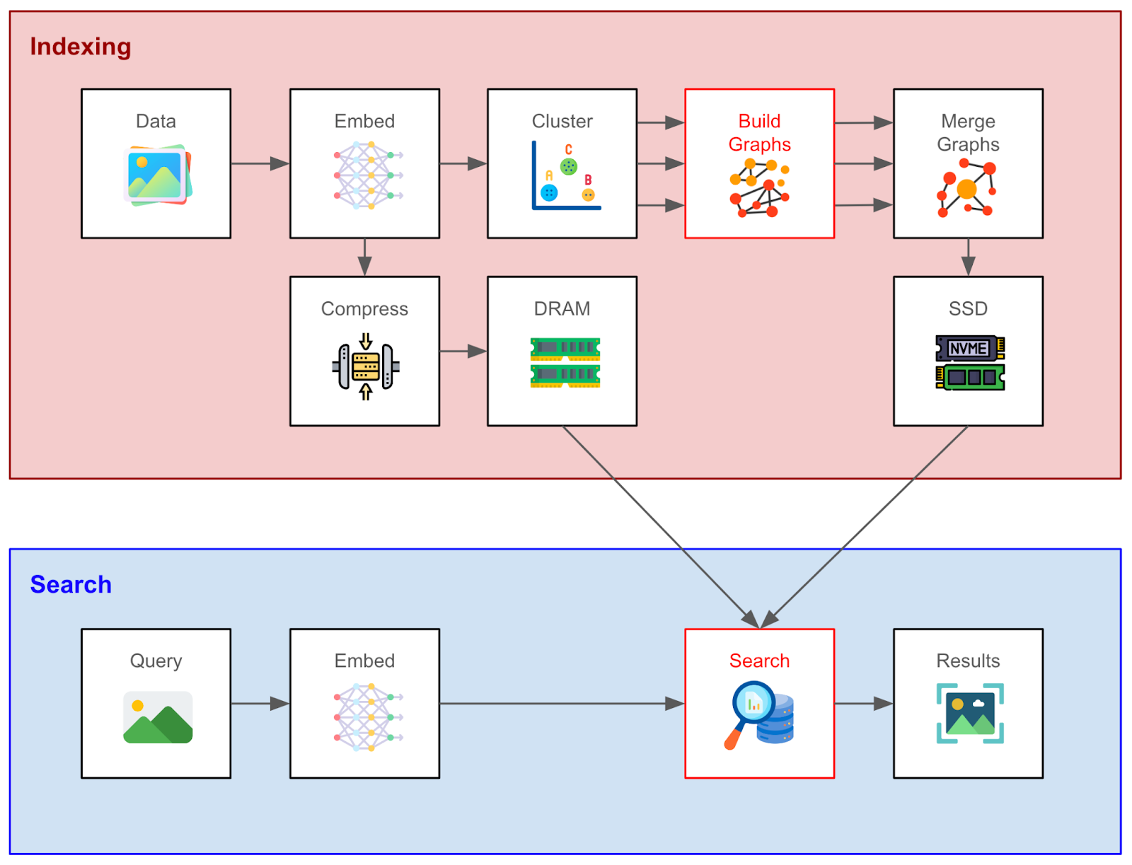
As modern artificial intelligence systems scale to ingest billions of multimodal embeddings, high-performance vector search and graph-based retrieval have transitioned from academic curiosities into foundational infrastructure components of enterprise data stacks. Whether powering semantic search engines, Retrieval-Augmented Generation (RAG) pipelines, or recommendation systems, the ability to query high-dimensional vector spaces with sub-millisecond latency is mission-critical. However, bridging the gap between theoretical research papers and production-grade software engineering remains one of the most perilous hurdles in systems architecture. Academic literature often relies on high-level mathematical abstractions and idealized pseudocode, leaving developers to discover critical memory-layout and data-structure bottlenecks only after shipping to production.
Key Technical & Architectural Takeaways
- Abstract Sets vs. Concrete Data Structures: Academic pseudocode references abstract sets like candidate lists and visited nodes. Translating these directly into naive collections (like unsorted vectors or dynamic hash maps) introduces catastrophic performance penalties, turning sub-millisecond approximate nearest neighbor searches into slower-than-brute-force bottlenecks.
- Bitset Acceleration for Visited Tracking: Replacing high-overhead hash sets with dense bitsets (such as boost::dynamic_bitset) for node traversal tracking eliminates heap allocations, slashes cache misses, and dramatically accelerates the innermost graph traversal loops.
- Logical vs. Physical Deletion: In high-throughput graph pruning routines, replacing costly physical deletions and memory shuffling with lightweight logical markers drastically reduces CPU overhead during hot-path execution.
- Massive Throughput Gains: Proper system-level mapping of the Vamana graph algorithm transforms indexing performance, shifting query execution times from 22.98 ms down to 0.02 ms while delivering over 5x the throughput of brute-force search at perfect recall.
- What is High-Performance Vector Search & Graph-Based Retrieval Systems?
- Deconstructing the Pseudocode-to-Production Gap
- Architectural Comparison: Graph Retrieval Implementation Strategies
- Deep Architectural Breakdown: Engineering the Vamana Search Loop
- Critical Evaluation & Real-World Trade-Offs
- Adoption Guide: When to Adopt vs When to Pass
- Strategic Architecture Conclusion & Production Roadmap
What is High-Performance Vector Search & Graph-Based Retrieval Systems?
High-Performance Vector Search & Graph-Based Retrieval Systems is a specialized class of algorithmic architectures designed to index, store, and query billions of high-dimensional vector embeddings by constructing proximity graphs that navigate semantic vector spaces with extreme computational efficiency and low query latency.
At its core, vector search addresses the fundamental challenge of finding the closest data points to a query vector in spaces scaling from dozens to thousands of dimensions. Traditional exact search methods, such as exhaustive linear scans, scale linearly with dataset size, rendering them economically and computationally infeasible for modern web-scale applications. To bypass this barrier, graph-based indexing algorithms—such as Hierarchical Navigable Small World (HNSW) graphs and the DiskANN Vamana graph—organize data points into proximity networks where edges connect mutually close neighbors. Query execution then boils down to a greedy search heuristic, hopping from node to node across the graph until it converges on the local neighborhood most similar to the query vector.
However, the transition from academic pseudocode to production code exposes a profound engineering disconnect. Papers describe components like candidate sets and visited registries as mathematical abstractions. Systems engineers must translate these abstractions into concrete physical memory layouts, cache-conscious data structures, and optimized concurrency models. Failing to bridge this gap correctly results in implementations that completely negate the theoretical speedups promised by graph algorithms.
Understanding High-Dimensional Proximity Graphs
To grasp why proximity graphs dominate the vector retrieval landscape, one must analyze the geometry of high-dimensional vector spaces. In spaces with hundreds or thousands of dimensions, traditional spatial partitioning trees (such as k-d trees or R-trees) break down due to the phenomenon known as the curse of dimensionality. In high dimensions, the distance between any two randomly chosen vectors tends to converge to a nearly uniform value, and partition boundaries inevitably overlap. Consequently, spatial trees degrade to exhaustive linear scans.
Proximity graphs circumvent this limitation by structuring the search space as a network of nodes connected by directed edges. The fundamental concept is to build a graph where the local neighborhood of each node represents its closest spatial neighbors. When searching, the engine initializes at an entry node and greedily traverses to the neighbor that is closest to the query vector. This path continues until no neighbor is closer to the query than the current node, representing a local minimum. To prevent the search from getting trapped in local minima that do not correspond to the true nearest neighbors, state-of-the-art algorithms introduce long-range edges, creating a “small-world” graph topology. This structural paradigm guarantees that any two arbitrary nodes in the graph can be connected by a small number of hops, mirroring the navigability of human social networks.
During a typical greedy search, the algorithm tracks two main concepts: routing through global cluster connectors (long-range edges) and clustering around local neighborhoods (short-range edges). Fast, hardware-level memory access is required to support these rapid hops across widely separated virtual memory addresses.
Deconstructing the Pseudocode-to-Production Gap
The pseudocode-to-production gap refers to the massive performance degradation that occurs when mathematical abstractions in academic papers, such as sets and unconstrained arrays, are directly implemented in code without optimizing for hardware-specific mechanics like CPU cache locality, memory layout, and SIMD instruction pipelines.
When studying seminal retrieval algorithms like DiskANN’s Vamana graph construction and search, engineers frequently encounter pseudocode that abstracts away underlying memory management. A typical search routine references abstract collections: a candidate set of nodes under consideration, a visited set to prevent redundant traversals, and dynamic neighbor lists. Treating these as generic collection types in high-level languages introduces subtle, compounding performance degradation.
Consider the candidate list. During a greedy graph traversal, the algorithm continuously inserts newly discovered neighbor nodes, sorts them by distance, prunes entries exceeding a fixed beam width or capacity bound, and extracts the closest unvisited node. Implementing this as a standard unsorted vector requiring a linear search for minimum extraction, followed by dynamic resizing and element shifting, introduces catastrophic CPU cache thrashing. Similarly, using standard hash-based sets (such as C++’s std::unordered_set or Python’s native set) for the visited registry forces continuous heap allocations, pointer chasing, and hash collision resolution inside tight loops.
The Reality of Hardware: CPU Caches and Memory Latency
Modern CPU architectures operate on hierarchical memory subsystems. While accessing data stored in registers takes less than a nanosecond, accessing main memory (DRAM) requires approximately 50 to 100 nanoseconds. To hide this latency, CPUs use L1, L2, and L3 caches, which pull in contiguous chunks of memory (64-byte cache lines) ahead of execution. When code is designed without consideration for these cache lines, the CPU frequently experiences cache misses, forcing it to stall while waiting for data to arrive from RAM.
A naive pointer-based graph implementation, where each node is allocated independently on the heap, scatters graph data across non-contiguous physical memory locations. As the search loop hops from one node to another, every edge traversal triggers a random memory lookup, leading to immediate L3 cache misses and Translation Lookaside Buffer (TLB) page walks. By contrast, production-grade vector databases pack nodes and their corresponding edge lists into aligned, contiguous byte arrays, optimizing sequential prefetching and spatial locality.
The following architectural pattern illustrates how abstract set concepts translate into naive, performance-inhibiting code versus cache-conscious production structures:
// NAIVE IMPLEMENTATION: High overhead, frequent heap allocations
#include <vector>
#include <unordered_set>
#include <algorithm>

struct NaiveNode {
    int id;
    std::vector<float> vector;
};

void naiveSearchStep(int candidateId, std::vector<int>& L, std::unordered_set<int>& V) {
    if (V.find(candidateId) == V.end()) {
        V.insert(candidateId);
        L.push_back(candidateId);
        // Expensive sorting on every insertion
        std::sort(L.begin(), L.end());
    }
}
In high-performance systems, every nanosecond counts. When query volumes reach tens of thousands of requests per second, heap-allocated hash maps and dynamic vector resizing become primary bottlenecks, starving the CPU pipeline and inflating tail latencies (p99 and p99.9 values).
Architectural Comparison: Graph Retrieval Implementation Strategies
Graph retrieval implementation strategies compare various structural approaches—such as memory-resident hierarchical graphs, flat list indexes, and disk-backed graphs—to balance query latency, index building time, RAM footprint, and recall accuracy. Choosing the correct strategy depends directly on dataset scale, hardware budgets, and latency SLAs.
To understand the design space of vector retrieval systems, it is instructive to compare naive academic implementations against optimized graph-based systems and alternative indexing paradigms like Inverted File Indexes (IVF) and Hierarchical Navigable Small Worlds (HNSW). Below is an architectural overview mapping out the physical characteristics, bottlenecks, and structural designs of each paradigm.
| Approach / Design | Latency / Throughput | Computational / Resource Complexity | Maturity | Best For |
|---|---|---|---|---|
| Naive Vamana Pseudocode Port | High Latency (~23ms per query), Lower throughput than brute force on small fixtures. | High CPU cache miss rate; frequent heap allocations and dynamic array resizing. | Experimental / Academic | Pedagogical understanding and algorithm verification only. |
| Optimized DiskANN (Vamana + Bitsets) | Sub-millisecond latency (~0.02ms), >5x throughput of brute force at 1.0 recall. | Low memory overhead; dense bitset lookups; cache-aligned structures. | Production-Grade | Large-scale, SSD-resident or RAM-resident multi-billion vector search. |
| HNSW (Hierarchical Navigable Small World) | Ultra-low latency, excellent recall. | High RAM consumption; index must reside entirely in volatile memory. | Industry Standard | In-memory vector search where RAM budget is not constrained. |
| IVF-PQ (Inverted File with Product Quantization) | Moderate latency, high throughput. | Low memory footprint due to lossy compression, requires periodic centroid training. | Mature | Memory-constrained environments willing to trade marginal recall for storage efficiency. |
Analyzing these models reveals that the HNSW graph provides outstanding performance for entirely in-memory datasets but scales poorly in terms of memory consumption, as it duplicates connections across hierarchical layers. IVF-PQ trades recall accuracy and query latency for a vastly reduced memory footprint by clustering vector spaces into centroids and compressing the residuals using Product Quantization. DiskANN’s Vamana graph bridges these worlds, offering a single-layer flat graph with wider reachability and a layout optimized to fetch nodes directly from SSD drives via asynchronous disk reads, yielding high performance without consuming massive amounts of RAM.
Deep Architectural Breakdown: Engineering the Vamana Search Loop
Engineering the Vamana search loop requires redesigning abstract mathematical traversals into low-level, cache-conscious systems code. By utilizing pre-allocated bounded arrays, lock-free concurrent structures, and dense bitsets instead of heap-allocated hashes, developers minimize memory latency and maximize SIMD vectorization during high-throughput graph navigation.
Achieving high-performance vector retrieval requires aligning code structures with underlying hardware architecture. Modern CPUs rely heavily on cache lines, spatial locality, and predictable branch prediction. To eliminate the performance pathologies of naive implementations, engineers must redesign core components to respect these hardware constraints.
1. Replacing Hash Sets with Dense Bitsets
In graph traversal algorithms, tracking visited nodes is executed millions of times per second. When node identifiers are dense integers (ranging from 0 to N – 1, where N is the total number of nodes in the graph), a hash table is entirely unnecessary and counterproductive. Replacing std::unordered_set with a dense bitset—such as boost::dynamic_bitset or a custom contiguous vector of 64-bit integers—reduces membership checking to a simple bitwise shift and mask operation.
#include <boost/dynamic_bitset.hpp>

class VisitedTracker {
private:
    boost::dynamic_bitset<>& visited_bits;
public:
    explicit VisitedTracker(boost::dynamic_bitset<>& bits) : visited_bits(bits) {}

    inline bool checkAndMark(size_t node_id) {
        if (visited_bits.test(node_id)) {
            return true; // Already visited
        }
        visited_bits.set(node_id);
        return false; // Newly visited
    }

    inline void reset() {
        visited_bits.reset();
    }
};
This optimization eliminates dynamic memory allocation during query execution, keeps working sets inside L1 and L2 CPU caches, and drastically reduces instruction cycles per graph hop.
2. Bounded Sorted Vectors for Candidate Management
Candidate lists in graph search must maintain a strict upper bound on size (beam width) while keeping elements sorted by distance to prioritize promising nodes. Instead of dynamic vectors with frequent insertions and deletions, a production-grade implementation utilizes a SortedBoundedVector struct. This data structure pre-allocates backing memory matching the maximum beam size and maintains sort order via insertion sort or binary search with fixed-size shifts.
#include <vector>
#include <algorithm>

struct Neighbour {
    float distance;
    uint32_t node_id;
    bool marked;

    bool operator<(const Neighbour& other) const {
        return distance < other.distance;
    }
};

class SortedBoundedVector {
private:
    std::vector<Neighbour> data;
    size_t capacity;
public:
    explicit SortedBoundedVector(size_t cap) : capacity(cap) {
        data.reserve(capacity);
    }

    bool insert(float dist, uint32_t id) {
        Neighbour n{dist, id, false};
        auto it = std::lower_bound(data.begin(), data.end(), n);

        // Check if already exists to prevent duplicates
        if (it != data.end() && it->node_id == id) {
            return false;
        }

        if (data.size() < capacity) {
            data.insert(it, n);
            return true;
        } else if (it < data.end()) {
            // Insert and trim excess capacity
            data.insert(it, n);
            data.pop_back();
            return true;
        }
        return false;
    }

    const Neighbour& operator[](size_t idx) const { return data[idx]; }
    size_t size() const { return data.size(); }
    void clear() { data.clear(); }
};
3. Logical Deletion vs. Physical Deletion
During graph pruning and dynamic index updates, nodes or edges are frequently removed. Physical deletion—splicing elements out of vectors and re-indexing adjacent pointers—introduces heavy memory movement overhead. Production graph engines implement logical deletion via marker flags (e.g., the bool marked field in the Neighbour struct). Hot traversal loops simply check the deletion flag and skip marked entries, deferring expensive compaction operations to asynchronous background maintenance threads.
4. Hardware-Level SIMD Optimization of Distance Metrics
To maximize search throughput, the innermost loops that compute distances between the query vector and neighbor candidate vectors must be accelerated using Single Instruction, Multiple Data (SIMD) instruction sets. In x86 architectures, AVX-512 and AVX2 allow the processor to execute operations on multiple floating-point values in a single clock cycle. Below is an optimized AVX2 implementation of Euclidean L2 distance for 32-bit floating-point vectors, which demonstrates how system level implementations completely bypass naive for-loops:
#include <immintrin.h>
#include <cstddef>

float avx2_l2_distance(const float* a, const float* b, size_t dimension) {
    // Process 8 float elements per iteration using 256-bit registers
    __m256 sum_vec = _mm256_setzero_ps();

    for (size_t i = 0; i < dimension; i += 8) {
        __m256 va = _mm256_loadu_ps(a + i);
        __m256 vb = _mm256_loadu_ps(b + i);
        __m256 diff = _mm256_sub_ps(va, vb);
        // Fused multiply-accumulate to accumulate squared differences
        sum_vec = _mm256_fmadd_ps(diff, diff, sum_vec);
    }

    // Horizontal addition of the 8 float components inside the register
    alignas(32) float buffer[8];
    _mm256_store_ps(buffer, sum_vec);

    float total_sum = buffer[0] + buffer[1] + buffer[2] + buffer[3] +
                      buffer[4] + buffer[5] + buffer[6] + buffer[7];

    return total_sum;
}
Replacing standard loop-based distance computations with vectorized AVX2 or AVX-512 code delivers a multi-fold speedup in the similarity search process. This ensures that memory bandwidth, rather than instruction throughput, remains the primary architectural scaling target.
Critical Evaluation & Real-World Trade-Offs
Evaluating graph-based vector search involves resolving fundamental trade-offs between RAM capacity, index build latency, and query execution speed. While memory-resident graphs offer the lowest latency, they require substantial hardware investments, forcing large-scale systems to adopt hybridized SSD-resident architectures like DiskANN to remain economically viable.
While optimizing data structures unlocks orders-of-magnitude performance gains, engineering teams must evaluate several critical trade-offs before deploying graph-based vector search systems to production:
- Memory Footprint vs. Query Latency: Graph indexes like Vamana and HNSW require storing adjacency lists alongside original vector embeddings. For massive multi-billion-scale datasets, maintaining the entire graph in RAM becomes cost-prohibitive, necessitating disk-based architectures (such as DiskANN) that leverage direct SSD access via asynchronous I/O frameworks like io_uring in Linux.
- Index Build Time Complexity: Constructing high-quality proximity graphs is computationally expensive. Unlike inverted indexes, which ingest data incrementally with minimal overhead, building a Vamana graph requires computing exact or approximate k-nearest neighbor graphs. This can take hours or even days for massive datasets, representing a substantial upfront compute investment.
- Parameter Sensitivity: Graph traversal performance is highly sensitive to hyperparameters such as candidate pool size during search and maximum graph node degree. Tuning these parameters requires balancing recall against query latency, demanding rigorous benchmarking across representative production query workloads.
- Concurrency and Thread Safety: Concurrent graph updates and searches require fine-grained locking or lock-free synchronization primitives. Poorly designed concurrency models lead to CPU pipeline stalls during edge pruning or deadlocks in multi-threaded query execution.
The Impact of Vector Quantization on Graph Performance
To mitigate the massive memory footprint of graph-based indexes, many systems employ vector quantization. Quantization converts high-precision 32-bit floating-point numbers into lower-precision representations, such as 8-bit integers (Scalar Quantization) or compressed codebook centroids (Product Quantization). While quantization drastically reduces memory consumption and accelerates SIMD distance calculations, it degrades the precision of distance computations. This degradation introduces errors in the greedy routing process, lowering the final recall. Production engines must navigate this trade-off by employing two-tier systems: utilizing quantized vectors to navigate the graph quickly, and using full-precision vectors to re-rank the final candidate list, achieving both high speed and high accuracy.
Adoption Guide: When to Adopt vs When to Pass
Determining whether to build a custom graph-based vector search system or adopt an off-the-shelf database depends on scale, latency constraints, and engineering resources. Teams with sub-millisecond SLA targets and specialized systems knowledge benefit from custom builds, while general applications should utilize database ecosystems.
To assist engineering leads and system architects in determining whether to invest in custom graph-based retrieval implementations or adopt established libraries, consider the following decision framework:
- Adopt Custom Graph Optimization When:
- Your application demands sub-millisecond query latencies at scale where existing managed solutions introduce unacceptable cost or latency overhead.
- You are operating in memory-constrained environments requiring tightly packed custom structs, zero-allocation traversal loops, and highly optimized embedded systems.
- Your team has deep systems programming expertise in C++ or Rust and understands CPU cache mechanics, assembly-level SIMD instructions, memory alignment, and system profiling tools like perf.
- You require deep vertical integration with specialized custom hardware accelerators, proprietary storage engines, or domain-specific distance metrics.
- Pass and Utilize Established Libraries When:
- You require rapid time-to-market and can leverage battle-tested vector databases (such as Milvus, Qdrant, FAISS, pgvector, or Pinecone) that have already solved these implementation hurdles.
- Your vector scale is modest (under tens of millions of items) where simpler indexing strategies (like IVF-FLAT or basic HNSW wrappers) satisfy your service level agreements.
- Your engineering organization lacks dedicated performance engineers to profile, debug, and maintain low-level memory allocators, concurrent graph modification routines, and custom bitset primitives.
Strategic Architecture Conclusion & Production Roadmap
A strategic production roadmap for high-performance vector search transitions from a profile-driven development phase to a hardware-optimized runtime environment. By prioritizing contiguous memory layouts, SIMD-accelerated distance computations, and lock-free concurrency, engineers can scale search infrastructure to sustain high-throughput, multi-billion vector retrieval workloads.
Translating academic algorithms into high-performance production software demands looking past the high-level abstractions of pseudocode and examining the physical realities of modern hardware. As demonstrated by optimizing the Vamana graph implementation from 22.98 ms down to 0.02 ms, performance bottlenecks rarely stem from algorithmic flaws; rather, they arise from mismatched data structures, excessive heap allocations, and cache-unfriendly memory layouts. By replacing abstract sets with dense bitsets, bounded sorted vectors, and logical deletion markers, systems engineers can unlock the full theoretical throughput of graph-based vector retrieval.
For engineering teams embarking on a vector search infrastructure project, the production roadmap should follow a phased approach: start by profiling baseline implementations using realistic workloads and representative datasets; replace dynamic collections with cache-conscious, pre-allocated data structures; introduce dense bitsets for visited state tracking; and rigorously benchmark recall-versus-latency trade-offs before scaling out. By adhering to these rigorous systems engineering principles, organizations can build robust, ultra-low-latency semantic retrieval engines capable of powering the next generation of artificial intelligence applications.